Risk Measures

Risk Functions

The main widely used risk measure for the instability and uncertainty of return over time is the variation over the expected return, which is the variance. There have been many discussions in recent years as to why standard deviation is not an appropriate measure of risk. Newer risk measures such as Value at Risk (Linsmeier and Pearson, 1996), Expected Tail Loss (Acerbi and Tasche, 2002), Omega ratio (Shadwick and Keating, 2002) and Maximum DrawDown (Chekhlov et al., 2005) are discussed and mathematically defined on this page.

Value at Risk (VaR)

Definition: \(VaR_\alpha\) is the minimum amount of money that is at risk when the investment is at the worst \(\alpha\%\) scenarios.

A mathematical definition of VaR is given as
\begin{equation} VaR_{\alpha}(S)=-\text{sup}\{x:\mathbf{P} [S < x]\leq \alpha\}, \end{equation} where \(S\) is the investment value that is considered to be a random variable.

Example: If \(VaR_{5\%}=400\) with daily data used in the calculations, then there is a worst case scenario with a 5% probability of loosing at least 400 in the next day.

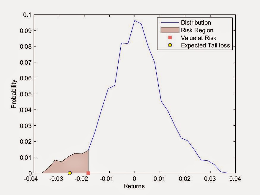
Figure1: VaR

Expected Tail Loss (ETL)

Definition: Expected Tail Loss is known as the Conditional Value at Risk ( \(CVaR_\alpha\)), which is defined as the expected loss given that the loss is beyond the \(VaR_\alpha\) of the investments.

A mathematical definition of CVaR is given below.

\begin{equation} CVaR_{\alpha}(S)=-\mathsf{E} [S|S\leq -VaR_{\alpha}(S)], \end{equation} where \(S\) is the investment value that is considered to be a random variable.

Example: \(CVaR_{3\%}=200000\) with monthly data used in the calculations means that the expected loss next month is 200000, given that the loss is known to be greater than or equal to the Value at Risk based on the worse 3% scenarios.

Figure2: VaR & CVaR

Omega \(\Omega\)

Definition: Omega risk measure is the ratio of expected (probability weighted) gains above a threshold to the expected (probability weighted) losses below the same threshold. Omega ratio \(\Omega\) is defined below and it represents the ratio of Area `B' to Area `A' in Figure 3. Bacmann and Scholz (2003) argue that the evaluation of an investment with the Omega ratio should be considered for thresholds between 0% and the risk-free rate.

\begin{align} \Omega(\tau)~ &\displaystyle{=\frac{\displaystyle{\int_\tau^\infty} [1-F(x)] \,\mathrm{d}x} {\displaystyle{\int_{-\infty}^{\tau}} F(x) \, \mathrm{d}x}},\\ &\\ &\displaystyle{=\frac{\text{Expected (probability weighted) gains above the threshold } \tau}{\text{Expected (probability weighted) losses below the threshold } \tau}}, \nonumber \end{align} where \(F(x)\) is the cumulative distribution function of returns and 0 is used as a threshold \(\tau\) .

Example: \(\Omega(0.02)=2.5\) tells us that the expected return exceeding 2% is 2.5 times the expected return less than 2% i.e.
$$ \displaystyle{\Omega(0.02)=\frac{E(r|r>0.02)-0.02}{0.02-E(r|r < 0.02)}\frac{1-F(0.02)}{F(0.02)}=\frac{\textrm{Potential Gain}}{~~\textrm{Potential Loss}}}. $$

Figure3: Expected (probability weighted) gain and loss areas

Maximum DrawDown (MDD)

Definition: Maximum DrawDown is the maximum loss (in percent) incurred over a given period for a buy-and-hold investor. Maximum DrawDown is defined below. \begin{equation} MDD=\displaystyle{ \max_{i,j}\frac{S_{i \in (0,T)}-S_{j \in (i,T)}}{S_i}}, \end{equation} where \(S_t\) is the asset price at time, \(t\in (0,T)\).

Example: \(MDD=\) 32% tells us that a maximum loss of 32% could happen if an investor has bought the security at peak and sold it at bottom that is the worst scenario in the holding period. 

Figure4: Maximum DrawDown for BP calculated over the period October 04, 2004 to December 04, 2007

---

References

1. Haidar, H., An empirical analysis of controlled risk and investment performance using risk measures: a study of risk controlled environment (Doctoral dissertation, University of Sussex, 2014).
2. Tang, Q., Haidar, H., Minsky, B., and Thapar, R. (2012). A Risk Measure for S-Shaped Assets and Prediction of Investment Performance. Journal of Financial Transformation, 34, 175-181.